Get Price
Double Beam UV Visible Spectrophotometer BSDBU-204-C
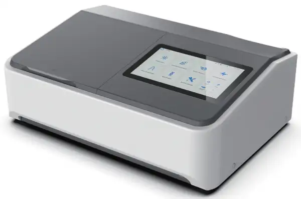
- • Large HD Smart Touch Screen
- High sensitivity and user-friendly UI for easy operation.
- • Stand-Alone System with Multi Functions
- Spectrum scanning, Standard curve, Kinetics, Multi wavelength, DNA/Protein test can be operated
- directly on device without PC software.
- • Automatic 8-position Cell Holder
- Higher efficiency of experiment to save time.
- • Easy Printing
 Get Quote
Specifications
| Model | BSDBU-204-C |
| Optical System | Double Beam |
| Light Source | W Lamp & D2 Lamp |
| Wavelength Range | 190-1100nm |
| Bandwidth | 0.5/1/2/4 nm |
| Display | 10-inch Touch Screen |
| Wavelength Accuracy | ±0.1nm at D2 656.1nm, ±0.3nm at full range |
| Wavelength Repeatability | ≤0.1nm |
| Photometric Accuracy | ±0.3%T (0-100%T); ±0.002Abs (0-0.5Abs); ±0.004Abs (0.5-1.0Abs) |
| Photometric Repeatability | ≤0.1%T (0-100%T); ≤0.001Abs (0-0.5Abs); ≤0.002Abs (0.5-1.0Abs) |
| Stability | ≤0.001A/h@250nm & 500nm, 2hrs warm-up |
| Photometric Range | -0.3-3A, 0-200%T, 0-9999C |
| Stray Light | ≤0.05%T at 220nm & 360nm |
| Control Mode | Stand-alone System or PC Software (Optional) |
| Data Output | USB Port or Bluetooth (Optional) |
| Power Requirement | AC 110/220V, 50/60Hz |
Features
High sensitivity and user-friendly UI for easy operation.
• Stand-Alone System with Multi Functions
Spectrum scanning, Standard curve, Kinetics, Multi wavelength, DNA/Protein test can be operated
directly on device without PC software.
• Automatic 8-position Cell Holder
Higher efficiency of experiment to save time.
• Easy Printing
Available to connect with general office printer directly (HP DeskJet 1111/1112/2723).
• USB Port, Fast Data Output
All test data can be exported to USB disk directly.
• Optional Bluetooth Module and PC software.
Bluetooth function and PC software are optional to meet different applications.
• Large Sample Chamber, Multi Options of Accessories
1-10cm universal cell holder, test tube holder, film holder, integrating sphere, specular reflectance accessory, peltier/sipper system, etc.
• High-quality Grating with High Performance
Lower stray light, higher stability and reliability.
• 16mm-thick Optical Base, Rigid Structure
All optical components are fixed on a 16mm thick rigid die-cast aluminum board to promise higher stability and reliability.
Items Included
| Name | Quantity | Unit |
| Spectrophotometer | 1 | unit |
| 1cm Glass cuvette | 4 | pcs |
| 1cm Quartz cuvette | 2 | pcs |
| Power cord | 1 | pcs |
| User's manual | 1 | pcs |
| Dust cover | 1 | pcs |
Operating Manuals
 Download Manual (PDF)
1. Introduction
1.1 Measurement Principle
1.2 Performance and features
1.3 Application
1.4 Technical Specifications
1.5 Packing List
1.6 Symbols and Notices
1.7 Product Design
2. Installation
2.1 Unpacking
2.2 Requirements
2.3 Installation
3. Instrument Operation
3.1 Power On & Self-diagnosis
3.2 Multi- cell Holder Management
3.3 Photometric Measurement
3.4 Quantitative Analysis
3.5 Kinetic Analysis
1. Introduction
1.1 Measurement Principle
The measurement principle of spectrophotometer is based on the Lambert-Beer law. When the beam of collimated monochromatic light passes through a certain uniform colored solution, the absorbance of the solution is directly proportional to the concentration of the solution and the optical path. And it supplies basis for the quantitative analysis. The Lambert-Beer law is described as following formula:
A=kbC
A - Absorbance of the analyte k - The absorption coefficient
b - The path length in cm
c - The analyte concentration
1.2 Performance and features
The performance and features of UV/Vis Spectrophotometer are as following:
▪ Low stray light and high resolution optical system enables accurate measurement with good stability and reproducibility.
▪ Novel technologies organically combine light, machine, electricity and microcomputer, together with scientific design, enables the instrument stability approaching or reaching a high level.
▪ 10 inches colorful capacitive touch screen, guarantees the touch point more precise, and enables much high sensitivity and excellent stability.
▪ High resolution with 1024 x 600, with fast running speed and large capacity.
▪ Interactive human machine interface enables the operation interface much friendly, and the operation is convenient.
▪ Powerful function of system settings, measurement functions such as photometric measurement, quantitative analysis, kinetic analysis, wavelength scan, multi- wavelength measurement, and DNA/protein measurement are available without on- line operation.
▪ Available for cell position control with the accessory of automatic cells holder.
▪ It provides unlimited storage. Data reading and writing are quite conveniently. USB storage is also available.
▪ Connecting to designated model of inkjet printer is available and with direct output of A4 paper report, enables the print report to be much neat and clear.
1.3 Application
The UV/Vis spectrophotometer is a common analytical instrument in chemistry laboratory, and it is widely used in pharmaceutical, medicine and health, chemical, energy, machinery, metallurgy, environmental protection, geology, food, biology, materials, agriculture, forestry, fisheries and many other industries. It's also applied in the fields of higher education, metrology, teaching and scientific research, and quality control, raw material and product inspection during production process.
Double beam UV/Vis spectrophotometers equipped with touch screen, thanks to their stable performance, accurate measurement and powerful functions, they have strong advantages in various fields of scientific research and quality control.
1.4 Technical Specifications
Model | BSDBU-204-C |
Wavelength Range | 190nm -1100nm |
Bandwidth | 0.5/1.0/2.0/4.0nm |
Wavelength Accuracy | ±0.3nm |
Wavelength Repeatability | ≤0.1nm |
Photometric Range | 0 - 200%T, -0.3A - 3A, 0 - 9999C |
Photometric Accuracy | ±0.3%T |
Stray Light | ≤0.05%T |
Dimensions | 610mm x 410mm x 230mm |
Table 1
1.5 Packing List
No. | Item | Unit | Qty | Note |
1 | UV/Vis Spectrophotometer | set | 1 | |
2 | Power Cord | pc | 1 | |
3 | Quartz Cell | kit | 1 | 2 pcs/kit |
4 | Glass Cell | kit | 1 | 4 pcs/kit |
5 | Dust Cover | pc | 1 | |
6 | User's Manual | pc | 1 | |
7 | Quality Certificate | pc | 1 | |
8 | Packing List | pc | 1 |
Table 2
1.6 Symbols and Notices
 : HIGH VOLTAGE.
Caution the danger of high voltage, and be careful of the risk of electric shock.
 : HOT SURFACE
Caution the hot surface, and avoid the risk of burn.
 : ULTRAVIOLET RADIATION
Caution the emission of UV radiation.
 : NOTICE.
Pay attentions to the notice.
 : SPECIAL EXPLANATION.
Pay additional attention to the special explanation.
1.7 Product Design
The profile of UV/Vis Spectrophotometer

Figure 1
The back side of UV/Vis Spectrophotometer

Figure 2
The compartment configuration of UV/Vis Spectrophotometer

Figure 3
Above figures are only for reference! Please refer to the actual configuration.
2. Installation
2.1 Unpacking
Please check the outer packing and make sure it is intact before unpacking. Then, check the instrument and accessories according to packing list and ensure they are completely well. If any questions, or anything lost or damaged, please contact us in time.
2.2 Requirements
A laboratory should be prepared, and following requirements should be met:
1) The instrument should be placed in a dry room, and the room temperature should be in the range of 5 °C- 35 °C. The relative humidity should be no more than 85%.
2) Power supply requirement: The rated voltage should be 220V ± 22V AC (110V ± 11V AC is also optional), the frequency should be 50Hz (60Hz is also optional). Well- grounded is also required. An electronic AC regulator or AC regulator with the power more than 1000W is suggested to enhance the anti-interference performance of the instrument.
3) Other requirements: Be far away from strong or continuous vibration. Neither setting up the instrument near electromagnetic field, nor exposing the instrument to direct sunlight or the radiation of heaters. It should be free of dust, as well as corrosive vapors. The instrument should be placed on a stable workbench. And for well cooling and ventilation, a clearance of at least 15 cm to the wall is suggested.
2.3 Installation
Install the instrument as following steps:
Step 1: Place the instrument onto a stable bench after unpacking.
Step 2: Connect the power cord to the instrument. If a printer is equipped, connect the power cord of the printer and connect the instrument to the printer with the communication cable.
3. Instrument Operation
Before switching on the device, make sure all connections working well. The power supply should be well-grounded and meet related requirements, neither sample in the sample compartment nor any other blocks in the light path.
Figures shown in this chapter are for reference only.
3.1 Power On & Self-diagnosis
1. Power On & Self-diagnosis
Switch on the device, it will proceed self-diagnosis. System will automatically diagnose the file, automatic sample holder, filter, tungsten lamp, deuterium lamp, lamp conversion, detector, Bluetooth, wavelength positioning, dark current, system parameters, and so on.

Figure 4
There is a status indicator lamp beside each self-diagnosis item, and it will turn green when the item passes in the self-diagnosis process. If any item is fail, the system will automatically give buzzing alarm, and the status indicator lamp will turn red at the same time. However, it will continue the self-diagnosis process.
Please don't open the lid of the sample compartment during the self-diagnosis process. Please contact us in time if any self-diagnosis item fails. Or refer to Chapter 5 for troubleshooting.
2. Warming up
Warming up starts after self-diagnosis finished, it takes around 20 min. The system will give buzzing alarm when warming up completed and enter the main operation interface automatically. Users also can click  to skip warming up.
3. Ready for operation
After warming up, device is ready for operation.
Functions such as photometric measurement, quantitative analysis, kinetic analysis, wavelength scan, multi-wavelength measurement, DNA/protein measurement and system settings are available, choose and click the icon accordingly to enter the related mode.

Figure 5
4. Description of touch keys
The common touch keys are shown on the bottom panel after entering each operation interface, followings are the descriptions.
 : For blank calibration, adjust to 0.000 Abs or 100.0 %T.
 : Save the data.
 : Open the data.
 : Exit the current interface, and return to the main interface.
 : Delete all records displayed in the current measurement interface.
 : Print the data.
 : For measurement parameters setting.
 : Measure and record the data.
 : Delete the selected measurement data.
 : Page up for data browsing or back to previous page.
 : Page down for data browsing or go to next page.
3.2 Multi- cell Holder Management
It's only available for the instrument with the accessory of certain automatic cell holder.
With the accessory of certain automatic cell holder, automatic measurement can be performed with functions of photometric measurement, quantitative analysis, multi- wavelength measurement, and DNA/protein measurement. Click the icon  on the
bottom right corner of the main interface to enter the multi-cell holder management
interface. User can choose manual or automatic operation mode with the multi-cell holder. If automatic mode is chosen, just select relevant cell positions and click  to return to the main interface, it will perform the measurement automatically after entering the specified measurement interface. If manual mode is chosen, after entering the specified measurement interface, click
  and click the corresponding position, the multi-cell holder will move to the right sample position and perform the measurement. User can measure other samples respectively by moving to certain sample position.

Figure 6

Figure 7
3.3 Photometric Measurement
Absorbance, transmittance, and energy measurements under certain wavelength are available with photometric measurement. The measurement result also can be printed out.
Click the icon  in the main interface to enter the photometric measurement interface.

Figure 8
If user want to change the test mode of current displaying shown in reading column, just click to enter the setting interface, select the test mode among Abs, T%, and E , then click to make sure the setting. Viewing the energy under certain wavelength with different gain is also available.

Figure 9
3.3.1 Photometric measurement
Following are the operation steps for photometric measurement. Step 1 Enter the photometric measurement interface.
Click the icon in the main interface to enter the photometric measurement interface.
Step 2 Set the measurement wavelength.
In the photometric measurement interface, click in the current wavelength display bar, a digital input window will pop up. Click  after inputting the wavelength value, a prompt "Moving wavelength …" will be shown, and the
instrument will move wavelength to the designated spot. User can click  to exit the digital input window if wavelength setting is unnecessary.

Figure 10
The valid wavelength range is between 190 nm and 1100 nm. If the input value is out of range, it is invalid, user needs to input again.
User can click to clear the input when an error is found, then input the target value again.
The touch key also works in the process of digital setting in subsequent operations.
Step 3 Sample measurement.
Put the blank solution or reference solution separately into the reference light path and sample light path, and click . The instrument will be adjusted to 0.000 Abs/100.0 %T under certain wavelength. Then, replace the blank solution or
reference solution with the sample solution only in the sample light path, click and record the measurement result.
3.3.2 Data processing
User can do data processing such as data saving, opening, printing and deleting after completing photometric measurements.
Data saving: User can save the data to the instrument memory by clicking . When a USB storage device is connected, user can select to save the data to the USB storage device. Input the file name in the file save window , and click , the file will be saved with the suffix of ".bas".

Figure 11
The valid length of the file name is no more than eight characters.
For data that already saved in the instrument memory, if user want to save it to the USB storage device later, please insert the USB storage device first. After opening the data in the instrument memory, long press and keep it for more than 3s before releasing, the file save prompts will pop up, select to save to the USB storage device, and then input the file name and confirm it, the data saving will be completed.
Data opening: Click to enter the data opening interface. User can select the file to be opened, and click to open the data.

Figure 12

Figure 13
Data printing: User can print the data by clicking if a printer is connected. A dialog box will pop up , click  to print the data.
Data deleting: If a few data need to be deleted, user can select the row of the data and click  at the bottom of the data sheet, a dialog box will pop up , click to make sure the deleting. User also can click on the lower pane of the
operation interface to clear all the data displayed in the data sheet. A dialog box will pop up , click to make sure the deleting.

Figure 14

Figure 15

Figure 13
The delete operation only works for current display. The already saved data won't lost. Before exit the current interface or returning to the main interface, a dialog box will pop up (Fig. 3-13). If the data after delete operation need to be saved, user can click to save the updated data.
3.4 Quantitative Analysis
User can do sample measurement based on the method of standard curve in the quantitative analysis interface. User also can utilize coefficient method to do sample measurement.
Click the icon  in the main interface to enter the quantitative analysis interface.

Figure 17
3.4.1 Standard curve measurement
The method of standard curve means to establish a calibration curve first, then measure the sample based on the calibration curve. The standard curve is also known as the standard calibration curve. Measure the absorbance of the sample and obtain the concentration that calculated according to the standard curve.
Different absorbance linearity range will cause different measurement error. The best absorbance linearity range is between 0.2 and 0.8.
1. Enter the interface of the standard curve method
In the main quantitative analysis interface, click  to enter the interface of the standard curve method.

Figure 18
2. Create standard curve
In the interface of the standard curve method, select the measurement method, set the wavelength, select the method "Std. Curve" and certain fitting method, set the std. number, and click to enter the standard curve measurement interface.
Following are detail operation steps for standard curve measurement: Step 1 Measurement method selection and wavelength setting.
There are two measurement method for chosen, single wavelength and dual wavelength. Click in the wavelength column in the interface of the standard curve
method, and a digital input window will pop up . Click after inputting the wavelength value. If the measurement method "Dual WL" is chosen, user
should input the calculation parameters after wavelength setting. Select the unit, there are six kinds of commonly used concentration unit for chosen, μg/L, mg/L, g/L, %, ppm and mol/L. Select the effective displaying of correlation coefficient. Click in std. number column, input the number value and confirm it. Then click to enter the standard curve measurement interface , a prompt "Moving wavelength …" will be shown, and the instrument will move wavelength to the designated spot.
Figure 19

Figure 20
Step 2 Standard samples measurement and standard curve establishing.
Click in the concentration column of std-1, input the concentration value and confirm it. Input other standard concentration value one by one. Put the reference solution of standard samples separately into the reference light path and sample light path, and click to adjust 0.000 Abs. Then, replace the reference solution
with the first standard sample solution only in the sample light path, click to record the Abs. value. Measure other standard sample solutions accordingly.
At last, the standard curve is obtained . Up to ten standard points can be measured.

Figure 21
Step 3 Sample measurement.
Click  in the obtained standard curve interface to enter the sample measurement interface. The curve information including the standard curve, curve equation and the correlation coefficient are shown on the left pane. Put the blank solution separately into the reference light path and sample light path, and click to adjust 0.000 Abs. Then, replace the blank solution with the sample solution only in the sample light path, click , the measurement result will be recorded.

Figure 22
In the sample measurement interface, user can click  to retrieve the data record of standard samples.

Figure 23
3. Data processing
User can do data processing such as data saving, opening, printing and deleting after completing standard curve measurement.
Data saving: User can save the data to the instrument memory by clicking . When a USB storage device is connected, user can select to save the data to the USB storage device. Input the file name in the file save window , and click , the file will be saved with the suffix of ".qua".

Figure 24
The valid length of the file name is no more than eight characters.
For data that already saved in the instrument memory, if user want to save it to the USB storage device later, please insert the USB storage device first. After opening the data in the instrument memory, long press and keep it for more than 3s before releasing, the file save prompts will pop up, select to save to the USB storage device, and then input the file name and confirm it, the data saving will be completed.
Data opening: Click to enter the data opening interface. User can select the file to be opened, and click to open the data.

Figure 25
Figure 26
Data printing: User can print the data by clicking if a printer is connected. A dialog box will pop up , click to print the data.
Data deleting: If a few data need to be deleted, user can select the row of the data and click at the bottom of the data sheet, a dialog box will pop up , click to make sure the deleting. User also can click on the lower pane of the operation interface to clear all the data displayed in the data sheet. A dialog box will pop up , click to make sure the deleting.
Figure 27
Figure 28
Figure 29
The delete operation only works for current display. The already saved data won't lost. Before exit the current interface or returning to the main interface, a dialog box will pop up (Fig. 3-26). If the data after delete operation need to be saved, user can click to save the updated data.
4. Load standard curve
User can load the saved standard curve. In the main quantitative analysis interface, click to  enter the standard curve loading interface

Figure 30
User can browse the pages by clicking and , and select the file of the standard curve need to be loaded. Then, click to enter the sample measurement interface.
The file are saved in ascending order, and the latest saved file is saved at the bottom. The instrument memory is unlimited, user can save files freely.
3.4.2 Coefficient method application
The coefficient method is a simple application of standard curve method. User can input the coefficients of the standard curve, and do the sample measurement further. The calculation formula is based on the fitting method. For linear fit, the calculation formula is C=K1xA+K0.
Following are detail operation steps for coefficient method:
Step 1 Enter the coefficient method interface.
In the main quantitative analysis interface, click to enter the interface of the standard curve method, select "Coefficient" as the method

Figure 31
Step 2 Measurement method selection and wavelength setting.
There are two measurement method for chosen, single wavelength and dual wavelength. Click in the wavelength column, and a digital input window will pop up. Click after inputting the wavelength value. If the measurement
method "Dual WL" is chosen, user should input the calculation parameters after wavelength setting. Then, select the unit. There are six kinds of commonly used concentration unit for chosen, μg/L, mg/L, g/L, %, ppm and mol/L.
Figure 32

Figure 33
Step 3 Coefficients setting.
For linear fit as an example, select the fitting method "Linear Fit". Click the blank column of K1, input the value in the pop-up digital input window and make sure the setting, input the value of K0 like the same. Then, click to enter the sample measurement interface (Fig. 3-30). A prompt "Moving wavelength …" will be shown, and the instrument will move wavelength to the designated spot.
Step 4 Sample measurement.
Put the blank solution separately into the reference light path and sample light
path, and click to adjust 0.000 Abs. Then, replace the blank solution with the sample solution only in the sample light path, click , the measurement result will be recorded.
User can do data processing such as data saving, printing and deleting after completing sample measurement. It is omitted here.
3.5 Kinetic Analysis
A curve of absorbance or transmittance or energy at a specific wavelength in a certain time range is available with kinetic analysis, and the variation tendency of a sample can be analyzed.
Click the icon  in the main interface to enter the kinetic analysis interface

Figure 34
3.5.1 Kinetic analysis
Following are the operation steps for kinetic analysis:
Step 1 Enter the kinetic analysis interface.
Click the icon in the main interface to enter the kinetic analysis interface.
Step 2 Set the kinetics scan parameters.
Click to enter the kinetics scan setting interface . User can select the test mode, set the measurement wavelength and time, time interval, the ordinate range. Click in the wavelength column, input the wavelength value in the digital input window, click to make sure the setting. Then, separately set the ordinate range and time like the same. Click to return to the kinetic analysis interface after completing all the settings.

Figure 35
The time interval can be selected among 0.5 s,1.0 s, 5.0 s, 10 s, 30 s, and 60 s.
Step 3 Kinetics scan.
Put the blank solution separately into the reference light path and sample light path, and click